Chatper 6 Partitioning

What is Partitioning

For very large datasets, or very high query throughput, we need to break the data up into partitions, also known as sharding.

What we call a partition here is called a shard in MongoDB, Elas‐ ticsearch, and SolrCloud; it’s known as a region in HBase, a tablet in Bigtable, a vnode in Cassandra and Riak, and a vBucket in Couchbase. However, partitioning is the most established term, so we’ll stick with that.

The main reason for wanting to partition data is scalability. Different partitions can be placed on different nodes in a shared-nothing cluster(sometimes called horizontal scaling or scaling out)

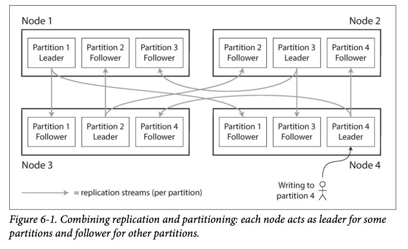
The choice of partitioning scheme is mostly independent of the choice of replication scheme, so we will keep things simple and ignore replication in this chapter

Partitioning of Key-Value Data

If the partitioning is unfair, so that some partitions have more data or queries than others, we call it skewed.

A partition with disproportion‐ ately high load is called a hot spot.

Partitioning by Key Range

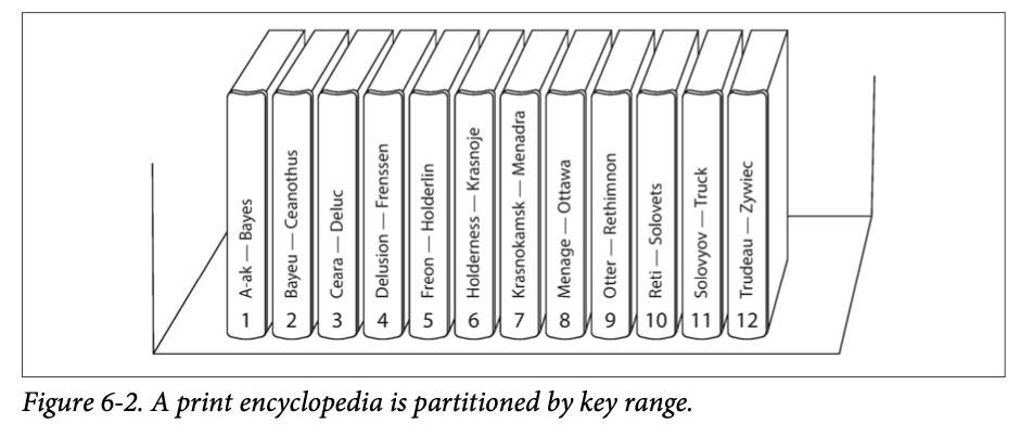
In order to distribute the data evenly, the partition bound‐ aries need to adapt to the data.

Within each partition, we can keep keys in sorted order

the downside of key range partitioning is that certain access patterns can lead to hot spots.

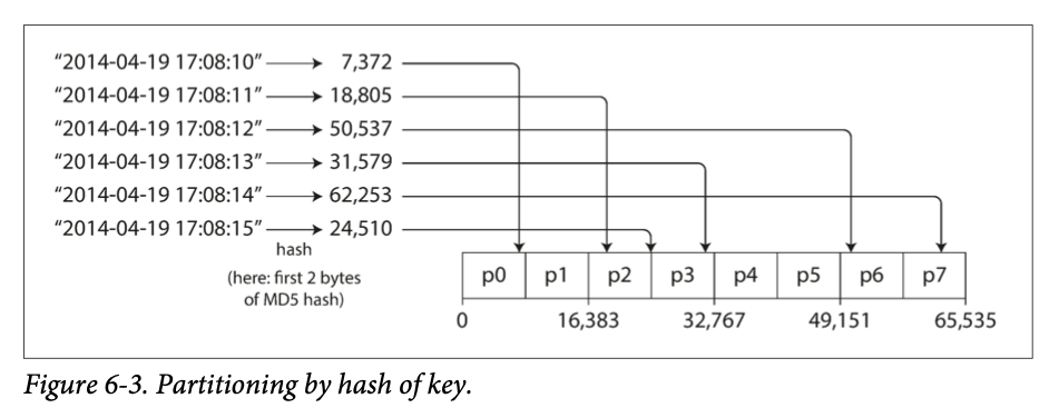
Partitioning by Hash of Key

For partitioning purposes, the hash function need not be cryptographically strong: for example, Cassandra and MongoDB use MD5, and Voldemort uses the Fowler– Noll–Vo function

Cassandra achieves a compromise between the two partitioning strategies [11, 12, 13]. A table in Cassandra can be declared with a compound primary key consisting of several columns. Only the first part of that key is hashed to determine the partition, but the other columns are used as a concatenated index for sorting the data in Cas‐ sandra’s SSTables. A query therefore cannot search for a range of values within the first column of a compound key, but if it specifies a fixed value for the first column, it can perform an efficient range scan over the other columns of the key.

CREATE TABLE sensor_data (
    location_id TEXT,        -- Partition Key
    timestamp TIMESTAMP,     -- Clustering Key
    temperature FLOAT,
    PRIMARY KEY (location_id, timestamp)
);

location_id | timestamp           | temperature
------------|---------------------|------------
A           | 2023-12-01 08:00:00| 22.5
A           | 2023-12-01 09:00:00| 23.0
A           | 2023-12-01 10:00:00| 21.8
B           | 2023-12-01 08:00:00| 19.5
B           | 2023-12-01 09:00:00| 20.0
 

valid:

SELECT * FROM sensor_data
WHERE location_id = 'A' AND timestamp > '2023-12-01 08:00:00';

invalid:

SELECT * FROM sensor_data
WHERE location_id > 'A';

What if partitioning by hash of key still introduce a skew? For example, a tweet of a celebrity.

Today, most data systems are not able to automatically compensate for such a highly skewed workload, so it’s the responsibility of the application to reduce the skew.

Just a two-digit decimal random number would split the writes to the key evenly across 100 different keys, allowing those keys to be distributed to different partitions.

This technique required additional bookkeeping to keep track of which keys are being split

Partitioning Secondary Indexes by Document

So far we’ve only covered the case where data is being accessed by primary key(car_id). What if we want to access data by secondary index(color)?

car_id	brand	model	color
1	Toyota	Corolla	red
2	Honda	Accord	blue
3	Ford	Mustang	red
4	Tesla	Model S	white

SELECT * FROM cars WHERE color = 'red';

each partition is completely separate: each partition maintains its own secondary indexes.
a document-partitioned index is also known as a local index

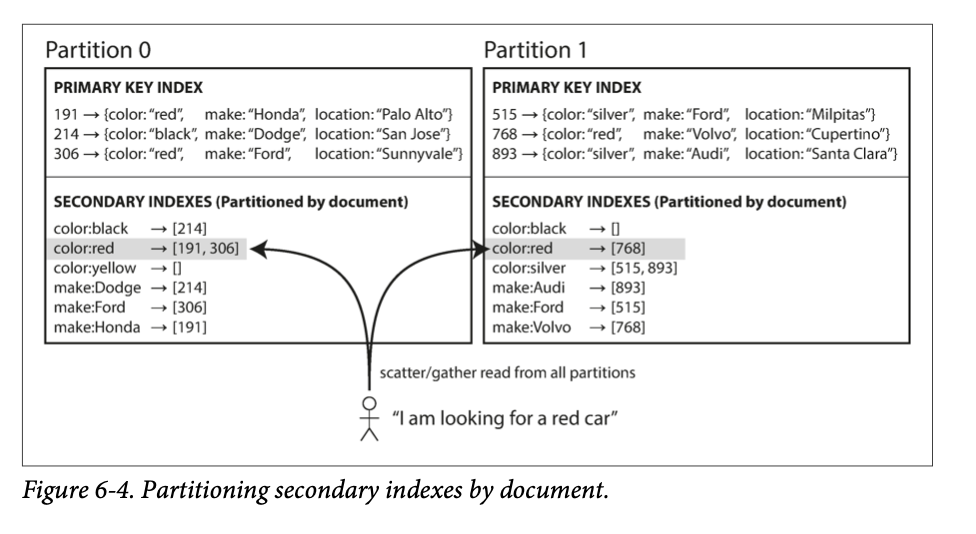if you want to search for red cars, you need to send the query to all partitions, and combine all the results you get back.

This approach to querying a partitioned database is sometimes known as scatter/ gather, and it can make read queries on secondary indexes quite expensive. Even if you query the partitions in parallel, scatter/gather is prone to tail latency amplification

Partitioning Secondary Indexes by Term

Rather than each partition having its own secondary index (a local index), we can construct a global index that covers data in all partitions.

Here we can partitioning by the term itself or the hash of the term, as discussed in the previous section.

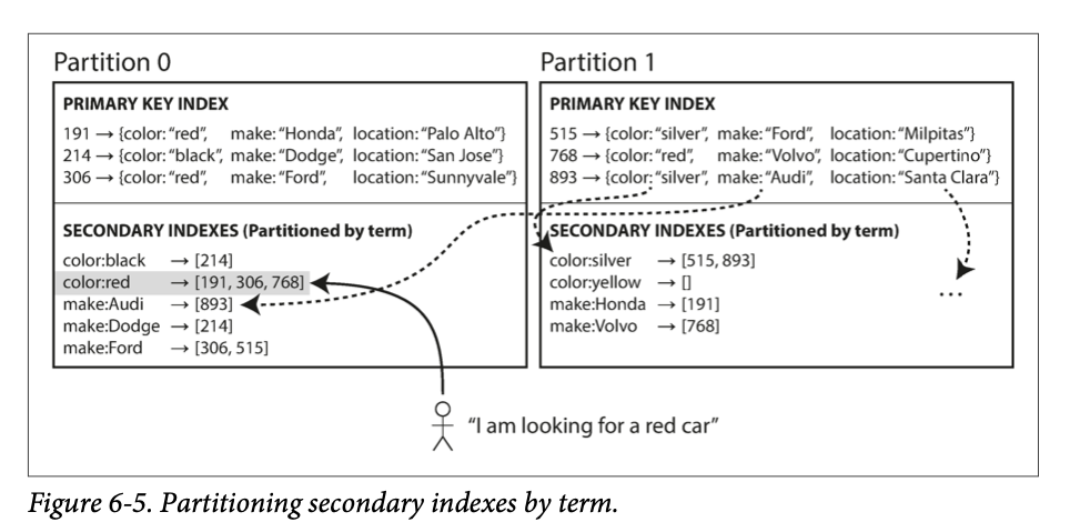
reads are more efficient, no scatter/gather over all partitions are needed. But writes are more expensive since it will affect multiple partitions of the index

Rebalancing Partitions

What if some machine fails, or to counter increasing dataset size or query throughput, more machines are added?

How not to do it: hash mod N → expensive for rebalancing

Fixed number of partitions

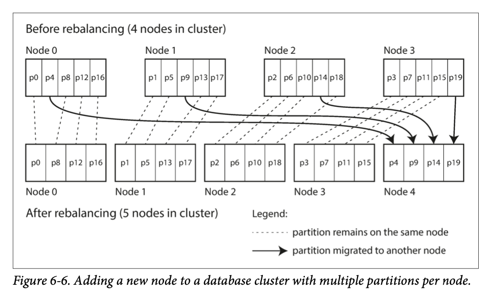
create many more partitions than there are nodes, and assign several partitions to each node

you can even account for mismatched hardware in your cluster: by assigning more partitions to nodes that are more powerful, you can force those nodes to take a greater share of the load.

Choosing the right number of partitions is difficult if the total size of the dataset is highly variable

Dynamic partitioning

When a partition grows to exceed a configured size (on HBase, the default is 10 GB), it is split into two partitions so that approximately half of the data ends up on each side of the split [26]. Conversely, if lots of data is deleted and a partition shrinks below some threshold, it can be merged with an adjacent par‐ tition. This process is similar to what happens at the top level of a B-tree (see “B- Trees” on page 79).

An advantage of dynamic partitioning is that the number of partitions adapts to the total data volume.

Dynamic partitioning is not only suitable for key range–partitioned data, but can equally well be used with hash-partitioned data.

Partitioning proportionally to nodes

make the number of partitions proportional to the number of nodes

When a new node joins the cluster, it randomly chooses a fixed number of existing partitions to split, and then takes ownership of one half of each of those split parti‐ tions while leaving the other half of each partition in place.

Picking partition boundaries randomly requires that hash-based partitioning is used

Consistent Hashing (virtual node) ???

compare it with Partitioning proportionally to nodes

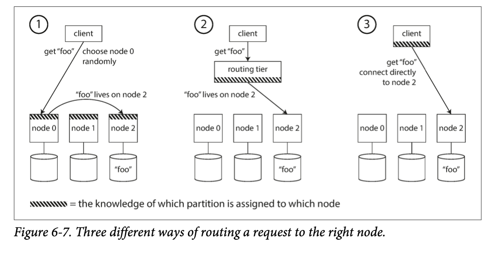
Request Routing

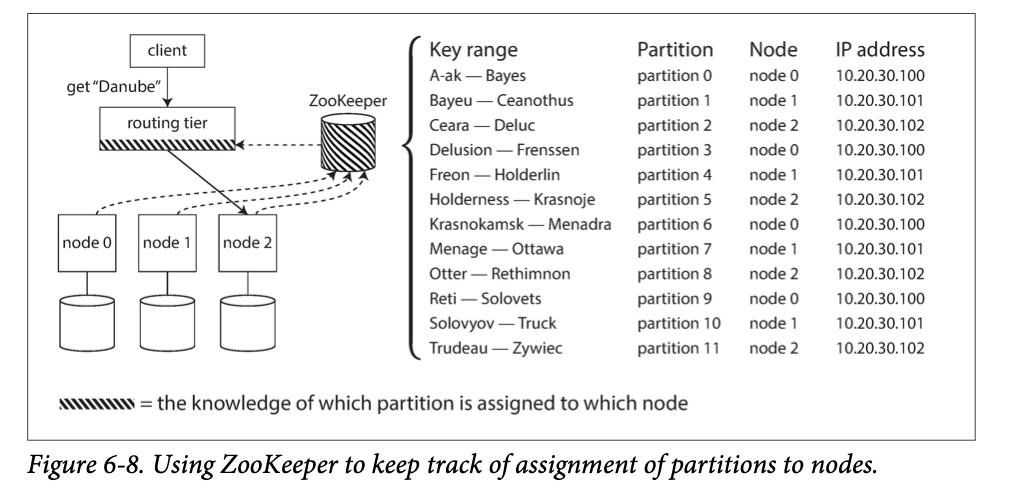
service discovery: how does the component making the routing decision (which may be one of the nodes, or the routing tier, or the client) learn about changes in the assignment of partitions to nodes?

ZooKeeper

Cassandra and Riak take a different approach: they use a gossip protocol among the nodes to disseminate any changes in cluster state.

Couchbase does not rebalance automatically, which simplifies the design. Normally it is configured with a routing tier called moxi, which learns about routing changes from the cluster nodes

Parallel Query Execution

massively parallel processing (MPP) Fast parallel execution of data warehouse queries → Chapter 10